Data Science Problem:

My project’s first objective was to predict the number of deaths from diseases related to air pollution: namely Ischaemic Heart Disease (IHD) and Chronic Obstructive Pulmonary Disease (COPD). The second objective was to isolate and quantify the effect of air pollution in those deaths. I decided to structure my problem so that I was predicting deaths for each five year age group (for example, 65-70 years) for each county in the continental United States.

Gathering Data:

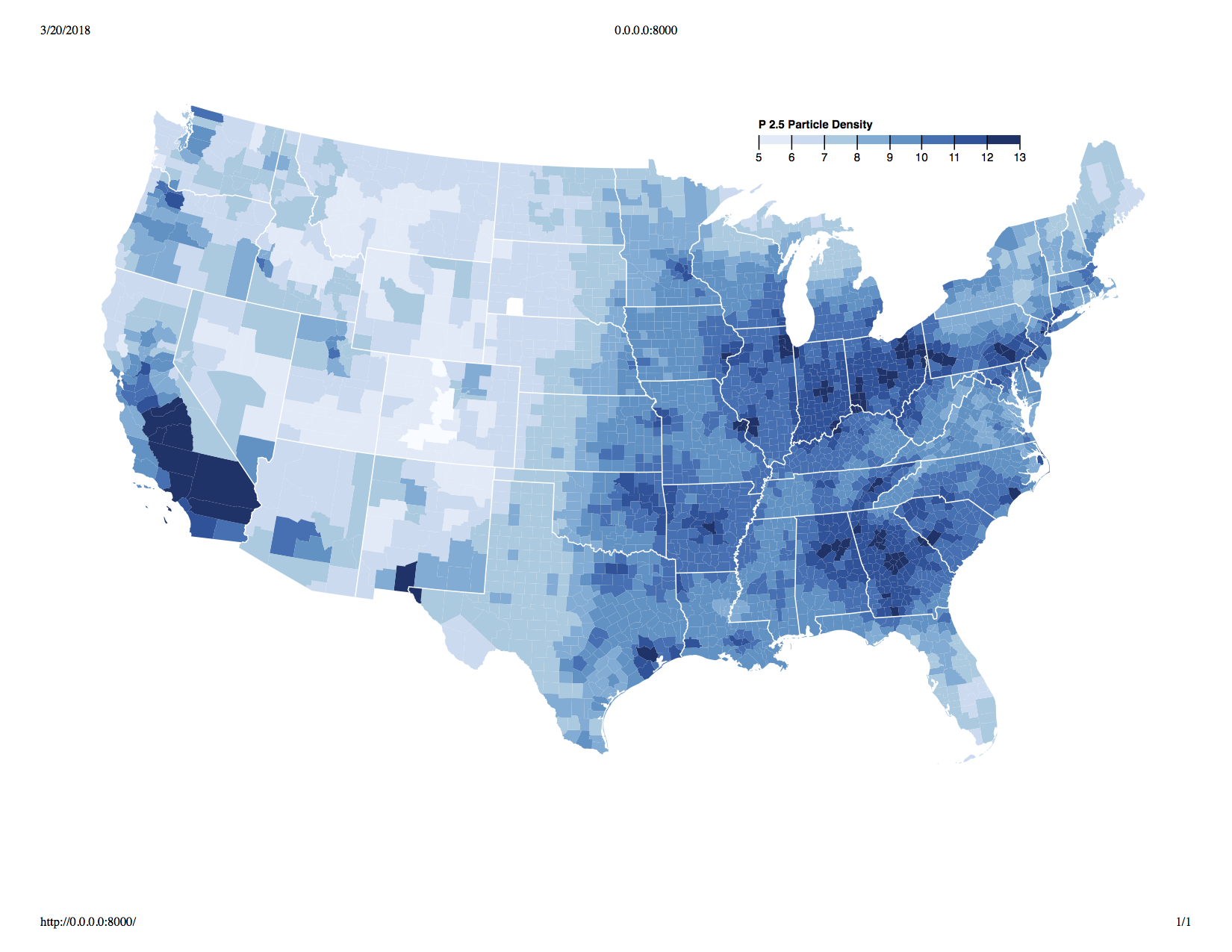
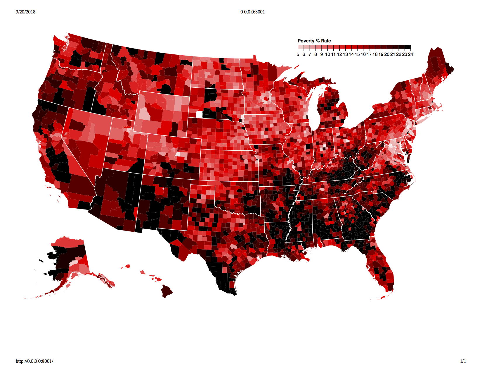
I gathered data on deaths by IHD and COPD from the Center for Disease Control for years ranging from 2001 to 2015. I found information on air pollution from the EPA website and used fine particulate matter (known as P_2.5 particles) density as a metric for air pollution. I also needed to control for confounders, so I looked at strong influencers of IHD and COPD such as obesity, % in poverty and size of metro (large metro, rural, etc.) among others, from a variety of sources.

One fear I had was that air quality would be highly correlated wth variables such as poverty, but a visual exploration showed that this was not necessarily the case. See below for the geographic distribution of air pulltion and % living in poverty:

Structuring Dataset:

I then picked four years for observing deaths (2012-2015). Following that, I looked at an eight year moving average of particle density and other features preceding the year of observed deaths. This is what my data set looked like:

• Observed deaths for 2015 - Average of features from 2004-2011
• Observed deaths for 2014 - Average of features from 2003-2010
• Observed deaths for 2013 - Average of features from 2002-2009
• Observed deaths for 2012 - Average of features from 2001-2008

I did this because a one year time lag of features (a regular time series) would not be a significant influence on deaths. For example, exposure to pollution must be continuous over a period of time, for it to take effect.

Selection of Models:

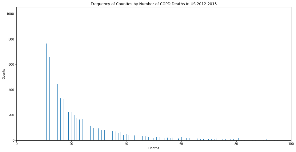
Let us focus on COPD for the remainder of this discussion. We will revisit IHD at the end of this post. I fitted my model on a training set using a Poisson GLM, since we are dealing with count data. The distribution of deaths against each age group shows that the Poisson GLM would be the most appropriate model to use.

With some regularization, I achieved good results (an R^2 of 0.70608 for COPD); while also achieving better results with a Random Forest regressor (R^2 of 0.87757 for COPD).

However, neither model could quantify the effect of particulate matter density reliably. With my Poisson GLM, the coefficient for this feature (variable) was small and fluctuated wildly based on the test train split. As for the Random Forest regressor, the model cannot provide coefficients to begin with (only feature importances). Since I clearly needed a different technique to quantify the effect of particle density, I tried controlling for confounders using K-Means.

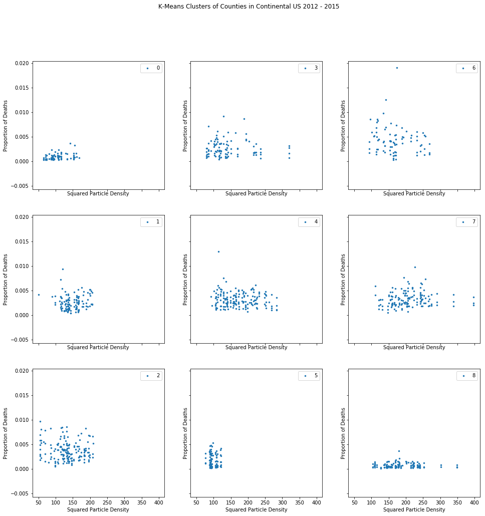
When that failed, I moved to a propensity score matching method, hoping for better luck in controlling for confounders.

Propensity Score Matching to Extract Effect of Pair Pollution:

First, I created two groups of counties as ‘high’ (high air pollution) and ‘low’ (low air pollution), separated by the median particle density for all counties. I then ran my features through a logistic regression classifier, asking it to predict if a county was ‘high’ or ‘low’, without having knowledge of death counts, nor actual particle density values. Below is the distribution of the two groups:

Since we have overlap between log likelihood of -1.8 and 0, we compare data points from both groupswithin that range. Note that the log likelihood for the ‘high’ safety group is concentrated near 0. This is expected, since predicitons for this group are much more accurate than the other group. I then received the likelihoods from the model, and matched pairs of counties - one to one - from the ‘high’ and ‘low’ groups. I matched them on their closeness in likelihood of having high pollution. This technique was essentially intended to create pairs of counties similar in every way except for death rates and particle density. In other words, it was an attempt to control of confounding variables.

We can then compare all possible pairs from each group, and retrieve pairs that have a ‘predict_proba’ output within .0005 of each other (in other words, very similar pairs). This should ensure that we have effectively controlled for confounders.

T-Test on Paired Data and Interpretation:

Finally, I ran a T-Test paired data (one variable being P_2.5 Density, and the other being the difference in proporition of deaths between pairs of counties). The p-vaule for this test is 0.02969; which is very low and, therefore, statistically siginficant. However, what about other variables? Are they statstically significant when paired with the attendance rate? If they were, it would mean that we had not yet effectively controlled for confounders. Let’s look at the p-values for other variables:

• % in Poverty: Ttest Result(statistic=-0.34819, pvalue=0.72785)
• Prevalence of Diabetes: Ttest Result(statistic=1.51644, pvalue=0.13006)
• Latitude: Ttest Result(statistic=-1.75320, pvalue=0.08020)
• Longitude: Ttest Result(statistic=1.58798, pvalue=0.11294)
• 2013 Urbanization Code: Ttest Result(1.57890, pvalue=0.11501)
• Population: Ttest Result(statistic=1.85492, pvalue=0.39302)

It is clear that P_2.5 Density was is the only statistically significant feature (meaning that air pollution does affect COPD death rates). I could see that, on average, counties with high particulate matter density witnessed more deaths by COPD than their low density counterparts. The actual difference was, on average, 7%, but we can only reject the null hypothesis here, and state that the mean difference is most likely not zero.

Further, although I found that the mean difference in death rates from COPD between pairs of ‘high pollution’ and ‘low pollution’ counties was statistically significant, for IHD it was not. For IHD we got -.007 as the mean difference between pairs. Not only is this difference very small, the differential is in the opposite direction to we were hoping for (fewer deaths in polluted counties)! The pvalue for this result was .89 which is far too close to 1 to attempt inference. This result looks very random, and not significant.

This makes intuitive sense, because the lungs are the first organs to be affected by air pollution, and not the heart! As an additional question, is there a sample size that would detect a mean difference of -.007 deaths fro IHD as significant?

Required Sample Size to Detect Significant Result for IHD:

The minimum sample size is related to the power of a test, which is the complement of a Type 2 error $(1-β)$. This is essentially probability of detecting a signficant difference between two statistics, if such a difference exists. If your (required) power is 80%, then this means that you have a 20% probability of failing to detect a significant difference when one does exist, i.e., a false negative result. It also means that you want 80% of the data points in your sampling distribution (i.e the 80th percentile of the distribution) to fall outside of the threshold of significance from your null distribution.

Let’s set $Zβ$ to be the z-score that marks the 80th percentile of the sampling distribution. This value is approximately .84 standard errors from the mean of the distribution. What about our threshhold for significance for the null distribution? Let’s set that at 5%. Let’s denote Zα to be the z-score marking the 97.5th percentile (since this is a two sided test) which roughly leads to 1.96 standard errors from the mean of the null distribution.

Putting all this together, we can say that we want 80% of the values from the sampling distribution to lie 1.96 standard errors away from the null distribution. The distance between the two means becomes our point estimate when we calculate our sample size. In other words, our point estimate is the z score from our threshold for significance plus our z-score from our power requirement (1.96 +.84 = 2.80).

Our margin of error is:

$(SE)\times(Zα+Zβ)$

where $SE$ in this case (0.0521) is the standard error of the sample of paired differences, and $(Zα+Zβ)$ is the point estimate.

However, we know we want our margin of error to be the difference between our mean difference between pairs (.007) and 0 (the null hypothesis): (.007-0).

Rearranging the equation:

$n = \frac{((Zα+Zβ)^2)\times VAR}{(.007-0)^2}$ where $VAR$ is the variance of our sample.

This is equal to a sample size of 2,030,376, which is much larger than we could possibly get in a real world setting!