This study looks at the relationship of different variables on attendance rates in NYC public high schools, and attempts to extract the effect of school safety in particular. Both school safety. as well as school attendance rates are both a critical focus for schools adiminstation entities.

The study uses five school years beginning 2006-2007, and contains the following variables:

• Academic Expectations
• Attendance Rate
• Communications
• DBN
• Engagement
• Enrollment
• Grade
• Overall Score
• Peer Index
• Percentile
• Principal
• Safety
• Weighted Environment
• Weighted Regents Pass Rate - English
• Weighted Regents Pass Rate - Math
• Weighted Regents Pass Rate - U.S. History

An intial look at the relationship between safety and attendance rates tells us that there some correlation between the two variables:

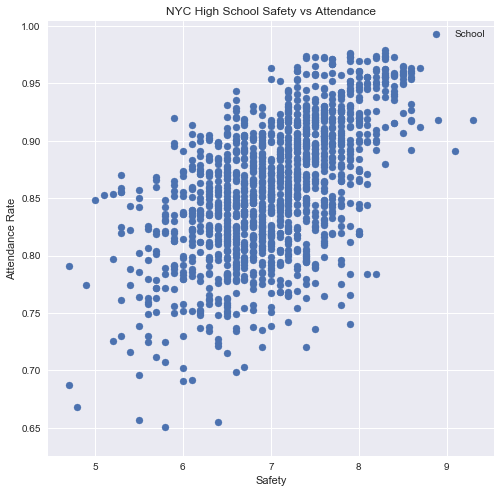
The R² for this relationship is at .33. However, we can safely say that many of the above variables are strongly co-dependent, so we can use K-Means to cluster the data points (data points being individual schools for a given year) into groups. This is carried out so that we can control for confounders correlated with safety. For this exercise, I have used nine groups.

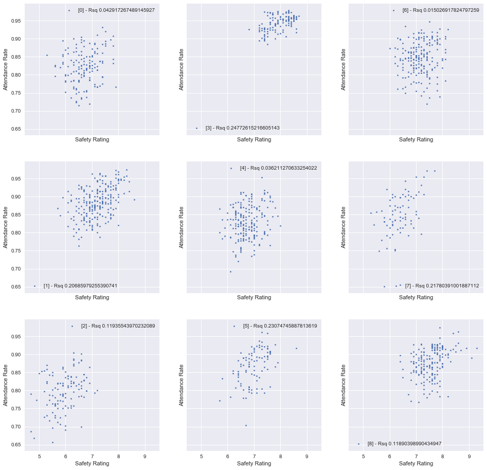
While the K-Means technique does still clearly show a relationship between safety and attendance (at least for some clusters), we would like to quantify the effect. With a maximum R² of around 30%, finding a linear relationship is not possible. Instead, we can approach this with a propensity score matching technique.

The objective of a propensity score matching technique is, once again, to control for all confounders. Do do this, we first create two groups of schools: ones with a low safety rating, and ones with a high rating. We can use the median score of 7 to create the separation.

Once this is done, we can run our data through logistic regression, asking the model to give us likelihoods of schools belonging to the ‘high’ and ‘low’safety groups based on the internal cost function. It should be noted that before running the model through logistic regression, we have to make the model blind to actual safety rating and attendance rates, since this will defeat the purpose of our classification.

For this classifification, I have used SciKit-Learn’s Logistic Regression algorithm, and generated likelihoods for each data point being in the ‘high’ or ‘low’ safety group based on the predict_proba output. Having done this, we can look at the pre-defined ‘high’ and ‘low’ groups (seperated earlier on median safety score of 7), and plot each data point’s likelihood of being in the ‘high’ safety group (irrespective of their manual classification).

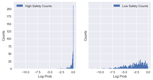
Since we have overlap between log likelihood of -2 and -.5, we compare data points from both groups within that range. Note that the log likelihood for the ‘high’ safety group is concentrated near 0. This is expected, since predictions for this group are much more accurate than the other group.

We can then compare all possible pairs from each group, and retrieve pairs that have a predict_proba output within .05 of each other (in other words, very similar pairs). This should ensure that we have effectively controlled for confounders.

Finally, we can do a t-test on paired data (one variable being safety, and the other being the attendance rate). The p-vaule for this test is 3.4495312085641958e-08; which is very and, therefore, statistically siginficant. However, what about other variables? Are they statstically significant when paired with the attendance rate? If they were, it would mean that we had not yet effectively controlled for confounders. Let’s look at the p-values for other variables:

• Enrollment: Ttest_relResult(statistic=-1.25784, pvalue=0.20924)
• Peer Index: Ttest_relResult(statistic=-1.05476, pvalue=0.29222)
• Academic Expectations: Ttest_relResult(statistic=2.40885, pvalue=0.01649)
• Communications: Ttest_relResult(statistic=-1.73013, pvalue=0.08444)
• Engagement: Ttest_relResult(statistic=1.24477, pvalue=0.21400)
• 4-Year Grad Rate: Ttest_relResult(statistic=-2.08667, pvalue=0.03760)
• Overall Score: Ttest_relResult(statistic=1.701660, pvalue=0.08965)
• Percentile: Ttest_relResult(statistic=1.42440, pvalue=0.15517)
• Weighted Environment: Ttest_relResult(statistic=-1.06625, pvalue=0.28700)
• Weighted Regent’s English: Ttest_relResult(statistic=1.65013, pvalue=0.099760)
• Weighted Regent’s Math: Ttest_relResult(statistic=2.125328, pvalue=0.03422)
• Weighted Regent’s US History: Ttest_relResult(statistic=2.29395, pvalue=0.02235)

Given that some of the other variables have p-values less than the standard of .05, we may say that we haven’t successfully controlled for confounders. This intuitively makes sense given that the means for attendance rates of the schools with high and low safety scores are as follows:

• Attendance rate for schools with ‘high’ safety scores: 0.84037
• Attendance rate for schools with ‘high’ safety scores: 0.85751
• Difference between means: -0.01713

It seems that we have achieved the opposite of what we set out to do! The propensity score matching technique tells us that schools with lower safety scores have higher attendance (albeit marginally). The fact remains that our results are inconclusive and, that by itself, a safety index does not have a (measurable) bearing on attendance rates.