
Finding the Line of Best Fit in Linear Regression using Different Methods
In this article we’ll come up with the line of best fit for linear regression using the least squares equation as well as the normal equation from linear algebra. While these methods are inter-connected, it is helpful to walk through the logic enshrined in the approaches. We’ll use SKLearn’s demo dataset ‘Boston’ for this purpose. We’ll then compare our values with SKLearn’s inbuilt LinearRegression class.
Import libraries and modules for use
import numpy as np
import matplotlib.pyplot as plt
import pandas as pd
from sklearn.datasets import load_boston
import seaborn as sns
from sklearn.linear_model import LinearRegression, SGDRegressor
Import dataset and check values
boston_dataset = load_boston()
boston = pd.DataFrame(boston_dataset.data, columns=boston_dataset.feature_names)
boston['MEDV'] = boston_dataset.target
boston.head()
| CRIM | ZN | INDUS | CHAS | NOX | RM | AGE | DIS | RAD | TAX | PTRATIO | B | LSTAT | MEDV | |
|---|---|---|---|---|---|---|---|---|---|---|---|---|---|---|
| 0 | 0.00632 | 18.0 | 2.31 | 0.0 | 0.538 | 6.575 | 65.2 | 4.0900 | 1.0 | 296.0 | 15.3 | 396.90 | 4.98 | 24.0 |
| 1 | 0.02731 | 0.0 | 7.07 | 0.0 | 0.469 | 6.421 | 78.9 | 4.9671 | 2.0 | 242.0 | 17.8 | 396.90 | 9.14 | 21.6 |
| 2 | 0.02729 | 0.0 | 7.07 | 0.0 | 0.469 | 7.185 | 61.1 | 4.9671 | 2.0 | 242.0 | 17.8 | 392.83 | 4.03 | 34.7 |
| 3 | 0.03237 | 0.0 | 2.18 | 0.0 | 0.458 | 6.998 | 45.8 | 6.0622 | 3.0 | 222.0 | 18.7 | 394.63 | 2.94 | 33.4 |
| 4 | 0.06905 | 0.0 | 2.18 | 0.0 | 0.458 | 7.147 | 54.2 | 6.0622 | 3.0 | 222.0 | 18.7 | 396.90 | 5.33 | 36.2 |
Description of data
print(boston_dataset.DESCR)
.. _boston_dataset:

Boston house prices dataset
---------------------------

**Data Set Characteristics:**

    :Number of Instances: 506

    :Number of Attributes: 13 numeric/categorical predictive. Median Value (attribute 14) is usually the target.

    :Attribute Information (in order):
        - CRIM     per capita crime rate by town
        - ZN       proportion of residential land zoned for lots over 25,000 sq.ft.
        - INDUS    proportion of non-retail business acres per town
        - CHAS     Charles River dummy variable (= 1 if tract bounds river; 0 otherwise)
        - NOX      nitric oxides concentration (parts per 10 million)
        - RM       average number of rooms per dwelling
        - AGE      proportion of owner-occupied units built prior to 1940
        - DIS      weighted distances to five Boston employment centres
        - RAD      index of accessibility to radial highways
        - TAX      full-value property-tax rate per $10,000
        - PTRATIO  pupil-teacher ratio by town
        - B        1000(Bk - 0.63)^2 where Bk is the proportion of blacks by town
        - LSTAT    % lower status of the population
        - MEDV     Median value of owner-occupied homes in $1000's

    :Missing Attribute Values: None

    :Creator: Harrison, D. and Rubinfeld, D.L.

This is a copy of UCI ML housing dataset.
https://archive.ics.uci.edu/ml/machine-learning-databases/housing/


This dataset was taken from the StatLib library which is maintained at Carnegie Mellon University.

The Boston house-price data of Harrison, D. and Rubinfeld, D.L. 'Hedonic
prices and the demand for clean air', J. Environ. Economics & Management,
vol.5, 81-102, 1978.   Used in Belsley, Kuh & Welsch, 'Regression diagnostics
...', Wiley, 1980.   N.B. Various transformations are used in the table on
pages 244-261 of the latter.

The Boston house-price data has been used in many machine learning papers that address regression
problems.

.. topic:: References

   - Belsley, Kuh & Welsch, 'Regression diagnostics: Identifying Influential Data and Sources of Collinearity', Wiley, 1980. 244-261.
   - Quinlan,R. (1993). Combining Instance-Based and Model-Based Learning. In Proceedings on the Tenth International Conference of Machine Learning, 236-243, University of Massachusetts, Amherst. Morgan Kaufmann.
EDA
Let’s designate ‘MEDV’ as our outcome variable. Let’s also use a correlation plot to find two variables with strong correlation with the outcome variable.
plt.figure(figsize=(10,10))
correlation_matrix = boston.corr();
# annot = True to print the values inside the square
sns.heatmap(data=correlation_matrix, annot=True,
            fmt='.2f',
            linewidths=.5,
            cmap="PuBu");
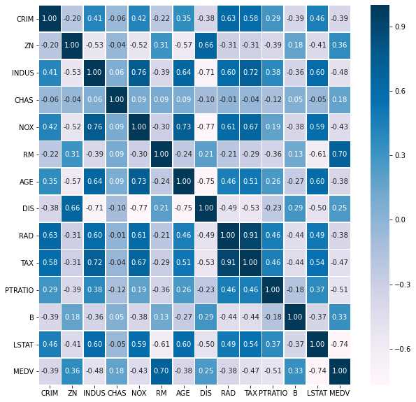
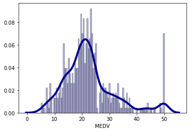
It seems that ‘RM’ and ‘LSTAT’ have a strong relationship with ‘MEDV’. Before we begin modeling, let’s look at the distribution of the outcome variable. Normality of the outcom variable is not a requirement for linear regression, but it typically helps. What is more important is that resuduals are normal. In the plot below, we can see that with the exception of high values, the data is fairly normally distributed.
sns.distplot(boston['MEDV'], hist=True, kde=True,
             bins=int(100), color = 'darkblue',
             hist_kws={'edgecolor':'black',
                       'alpha':.3},
             kde_kws={'linewidth': 4});
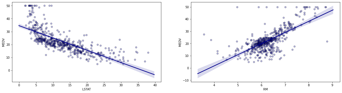
Let us try to construct the line of best fit between ‘MEDV’ and each of our chosen predictors (‘LSTAT’ and ‘RM’). The line of best fit is given by:
The expected value for the outcome variable are given by:
where $\beta_0$ and $\beta_1 $ are unkown parameters. Let’s look at the lines of best fit for each of our models using Seaborn’s inbuilt functionality
Plotted lines of best fit with data
fig, (ax1, ax2) = plt.subplots(1,2, figsize=(20, 5));
sns.regplot(boston['LSTAT'],
            boston['MEDV'],
            ax=ax1,
            scatter_kws={'edgecolor':'black',
                         'alpha':.3},
            color='darkblue');
sns.regplot(boston['RM'],
            boston['MEDV'],
            ax=ax2,
            scatter_kws={'edgecolor':'black',
                         'alpha':.3},
            color='darkblue');
Residual Plots
fig, (ax1, ax2) = plt.subplots(1,2, figsize=(20, 5));
sns.residplot(boston['LSTAT'],
            boston['MEDV'],
            ax=ax1,
            scatter_kws={'edgecolor':'black',
                         'alpha':.3},
            color='darkblue');
sns.residplot(boston['RM'],
            boston['MEDV'],
            ax=ax2,
            scatter_kws={'edgecolor':'black',
                         'alpha':.3},
            color='darkblue');
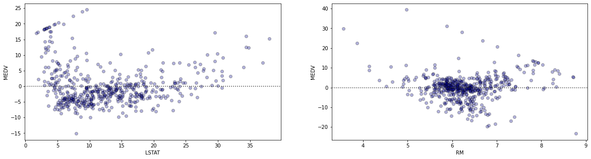
Given that the residuals are not normally distributed, it would be difficult to interpret the p-values associated with our coefficients. However, the purpose of this exercise is not to look at p-values, but the different approaches to generating the coefficients. In our first set of plots with the lines of best fit, pay attention to the each of the data points scattered around each of the regression lines. The vertical distances between each of the datapoints and the line of best fit become the errors for those data points. When we square these errors and sum them up, we get the residual sum of squares $\sum_{i=1}^n(y_i - \hat{y_i})^2$. Therefore, the residual sum of squares $(RSS)$ becomes:
$RSS$ is minimized with respect to $b_0$ and $b_1$ when:
Rearranging these equations gives
and
Solving these gives the least squares estimates.
For the intercept:
and the slope:
With respect to the above dataset, we can find the $\hat{\beta_1}$ using the above equation:
beta_1 = ((boston['LSTAT'] -
           boston['LSTAT'].mean())*(boston['MEDV'] -
                                    boston['MEDV'].mean())).sum()/((boston['LSTAT'] -
                                                                    boston['LSTAT'].mean())**2).sum()

beta_1
-0.9500493537579907
Recall from above that we can find the intercept using $\hat{\beta_0} = \bar{y} - \hat{\beta_1}\bar{x}$
beta_0 = boston['MEDV'].mean() - beta_1*boston['LSTAT'].mean()

beta_0
34.5538408793831
We can verify our results using SKLearn’s LinearRegression class. The class uses Scipy’s least squares solver (normal equation)
lr = LinearRegression()

lr.fit(boston[['LSTAT']],boston['MEDV'])

lr.intercept_, lr.coef_[0]
(34.5538408793831, -0.9500493537579906)
We can see that the two methods provide the same results. Let’s do the same for the predicted variable ‘RM’
beta_1 = ((boston['RM'] -
           boston['RM'].mean())*(boston['MEDV'] -
                                    boston['MEDV'].mean())).sum()/((boston['RM'] -
                                                                    boston['RM'].mean())**2).sum()

beta_0 = boston['MEDV'].mean() - beta_1*boston['RM'].mean()

beta_0, beta_1
(-34.67062077643857, 9.10210898118031)
lr = LinearRegression()

lr.fit(boston[['RM']], boston['MEDV'])

lr.intercept_, lr.coef_[0]
(-34.67062077643857, 9.10210898118031)
Normal Equation Approach
Let’s dive into the mechanics of the normal equation referenced above. The least squares equation can be generalized using matrix algebra which will allow us to solve multiple equations for a large featurespace at once. Let’s look at the equation $Ax = b$ where $A$ is an $m \times n$ matrix and $b$ is a vector in $\mathbb{R}^m$. The least squares solution is given by
This is equivalent to a vector $\bar{y}$ in the column space of A such that:
for all $y$ in the column space of $A$ ($col(A)$)
If $\bar{x}$ is the least squares solution of $Ax = b$, then:
We know that if $proj_{col(A)}(b)$ is the projection of $b$ onto the column space of $A$ and $perp_{col(A)}(b)$ is the error vector perpendicular to $col(A)$:
Therefore $b- A\bar{x} $ is in the nullspace of $A^t$. As a result:
This is equivalent to
Rearranging this gives us:
To find the least squares solution:
Let’s do this for a single predictor for now
boston['intercept'] = 1

A = np.array(boston[['intercept','RM']])
B = np.array(boston['MEDV'])

# Generate least squares solution
C = np.matmul(np.linalg.inv(np.matmul(np.transpose(A),A)),(np.transpose(A)).dot(B))

C
array([-34.67062078, 9.10210898])
Let’s now try the same for a multivariate model:
lr = LinearRegression()

lr.fit(boston[['RM', 'LSTAT']], boston['MEDV'])

lr.intercept_, lr.coef_
(-1.358272811874489, array([ 5.09478798, -0.64235833]))
A = np.array(boston[['intercept','RM','LSTAT']])
B = np.array(boston['MEDV'])

C = np.matmul(np.linalg.inv(
              np.matmul(np.transpose(A),A)),
              (np.transpose(A)).dot(B))

C
array([-1.35827281, 5.09478798, -0.64235833])
As we can see, SKLearn’s LinearRegression package gives us the same results as our constructed normal equation