Poisson Regression and Intuition Behind Poisson Distribution of Y Variable

In Poisson regression, we assume that our Y variable is Poisson distributed. This means that we assume that each row in the dataset is Poisson distributed with its unique expected value.

In other words, the expected value for each row is $\lambda =\operatorname {E} (Y\mid x)=e^{\theta ‘x}$ where $\theta$ is our set of coefficients and $x$ is our feature space. However, in many datasets where Y is Poisson distributed, The $Y$ vector itself is Poisson distributed, even though each observation presumably has its own unique $\lambda$ parameter. Let’s explore why this might be the case. A primer on the Poisson random variable and the Poisson regression are given at the end of this notebook under sections:

Poisson Random Variable
Poisson Regression and log link function

In the meantime, let’s explore a contrived dataset.

Import libraries and modules for exploration

import numpy as np
import warnings 
warnings.filterwarnings('ignore')
import pickle
import pandas as pd
import seaborn as sns; sns.set(color_codes=True)
import pandas as pd

Let’s create a dataframe from random randomly from a range

df = pd.DataFrame({'x': np.random.normal(500, 250, 100000),
                   'y': np.random.normal(500, 250, 100000),
                   'z': np.random.normal(500, 250, 100000)})

Let’s also create an outcome variable using a random linear regression equation applied to our randomly generated featurespace

df['outcome'] = df['x']*.003+df['y']*.001+df['z']*.0006

Let’s the resulting outcome

sns.kdeplot(df['outcome'],
            shade=True);

png

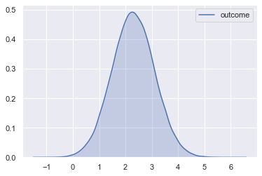
We can see that the outcome variable is fairly symmetric. Let’s treat each row’s outcome as an expected value from a Poisson distribution and draw a random value from each distribution. Notice that we have to exponentiate the outcome variable. See the end of the notebook on Poisson regression for more information.

df['outcome'] = np.exp(df['outcome']).apply(lambda x: np.random.poisson(x))

sns.kdeplot(df['outcome'],
            shade=True);
plt.xlabel('Value of Observation');
plt.ylabel('Density / Normalized Count');
plt.xlim(0,60);

png

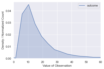
Now we can see that the fairly symmetric shape now has a distinct Poisson flavor. Why is this? This is because we have multiple Poisson distributions overlaid, which means the final curve is informed by those individual Poisson curves. The only way to visualize this is to take small windows of the featurespace, and plot each window. This means that each window will have a set of $\lambda$ values that are very close to each other.

fig, ax = plt.subplots(1,2,figsize=(15,5))
for i,j in [(0,200),
            (200,400),
            (400,600),
            (600,800)
            ]:
    hist_series = df[(df['x']>i) & 
                     (df['x']<j) &
                     (df['y']>i) &
                     (df['y']<j) &
                     (df['z']>i) &
                     (df['z']<j)]['outcome']
    
    sns.kdeplot(hist_series,
                    shade=True, 
                    label='{} < Featurespace < {}'.format(i,j),
                    ax=ax[0])
    sns.kdeplot(hist_series,
                    shade=True, 
                    alpha=.1,
                    label='{} < Featurespace < {}'.format(i,j),
                    ax=ax[1])
    
    
sns.kdeplot(df['outcome'],
             ax=ax[1]);                  
ax[0].set_xlabel('Value of Observation');
ax[1].set_xlabel('Value of Observation');
ax[0].set_ylabel('Density / Normalized Count');
ax[0].set_title('Partitioned KDE');
ax[1].set_title('Full KDE');
ax[1].set_xlim(0,60);

png

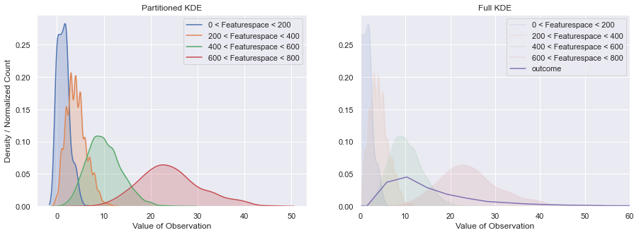
From the above plot it is evident that individual outcomes are relatively small (closer to zero) and indeed come from Poisson distributions, the outcome vector as a whole will follow the shape of the Poisson distribution as well. for those who would like a refresher on both the

Poisson Random Variable

The Poisson random variable is used to model count data. The probability mass function for a Poisson random variable is given as:

$p(k) = \frac{\lambda^k e^{-\lambda}}{k!}$

Where ${\lambda}$ is the mean or expected value of the Poisson random variable and k is the observed outcome. ${p(k)}$ tells us the probability of observing such an outcome given ${\lambda}$. Let’s set about deriving the above pmf. Let’s start with defining our expected value. Recalling the binomial distribution, we can model the expected value as:

$E(X) = \lambda = np$

Where E(X) is the expected value of the Poisson random variable, n is the number of trials, and p is the probability of success in a given trial. Then, as per our binomial distribution, the probability of k outcomes in n trials will be:

$P(X = k) = {n \choose k}(\frac{\lambda}{n})^{k}(1-\frac\lambda{n})^{(n-k)}$

However, in order to ensure $k$ successes and not more than $k$ successes, we have to get very granular, and ensure the intervals $n$ are as large as possible. Therefore, we send $n$ towards infinity.

$P(X = k) = \lim_{n\to\infty}{n \choose k}(\frac{\lambda}{n})^{k}(1-\frac\lambda{n})^{(n-k)}$

We can also separate exponent terms to make them easier to wield:

$P(X = k) = \lim_{n\to\infty}\frac{n!}{(n-k)!k!}(\frac{\lambda}{n})^{k}(1-\frac\lambda{n})^{(n)}(1-\frac\lambda{n})^{(-k)}$

Now, when ${n\to\infty}$, $\frac{n!}{(n-k)!}$ $\to\ 1$. Also $(1-\frac\lambda{n})^{(-k)}$ $\to\ 1$.

Now, can we recall the relationship between our number of trials $n$ and $e$?

Let’s look at the relationship between $n$ and $e$:

$\lim_{n\to\infty}(1+\frac1n)^n \simeq e$ $\lim_{n\to\infty}(1+\frac{a}n)^n \simeq e^{a}$ $\lim_{n\to\infty}(1-\frac{a}n)^n \simeq e^{-a}$

Therefore:

$(1-\frac\lambda{n})^{n}\to\ e^{-\lambda}$ .

Substituting all of these values in our equation, we get

$p(k) = (1)\frac{\lambda^k e^{-\lambda}}{k!}(1)$

$p(k) = \frac{\lambda^k e^{-\lambda}}{k!}$

Poisson Regression and log link function

Now, Poisson regression is a generalized linear model. It assumes the $Y$ variable is Poisson distributed and, if the canonical log link is used, that log value of $Y$ can be modeled by a set of linear predictors. Read the Wikipedia page for more information.

Under this model, $\lambda$ (expected value) is represented as follows:

$\lambda =\operatorname {E} (Y\mid x)=e^{\theta ‘x}$ where $\theta$ represents our vector of coefficients and $x$ represents our feature space.

Therefore our probability mass function becomes: $p(y\mid x;\theta )={\frac {\lambda ^{y}}{y!}}e^{-\lambda }={\frac {e^{y\theta ‘x}e^{-e^{\theta ‘x}}}{y!}}$

Then our likelihood estimate becomes:

$p(y_{1},\ldots ,y_{m}\mid x_{1},\ldots ,x_{m};\theta )=\prod _{i=1}^{m}{\frac {e^{y_{i}\theta 'x_{i}}e^{-e^{\theta 'x_{i}}}}{y_{i}!}}$ $L(\theta \mid X,Y)=\prod _{i=1}^{m}{\frac {e^{y_{i}\theta 'x_{i}}e^{-e^{\theta 'x_{i}}}}{y_{i}!}}$

However the above product form becomes unwieldy and computationally expensive, so we use log likelihood instead. As can be seen from the equation below, log likelihood is elegant:

$\ell (\theta \mid X,Y)=\log L(\theta \mid X,Y)=\sum _{i=1}^{m}\left(y_{i}\theta 'x_{i}-e^{\theta 'x_{i}}-\log(y_{i}!)\right).$

Now, notice that that $-\log(y_{i}!)$ does not depend on $\theta$, therefore, we can remove it from the objective function.

$\ell (\theta \mid X,Y)=\sum _{i=1}^{m}\left(y_{i}\theta 'x_{i}-e^{\theta 'x_{i}}\right)$

In order to find the maximum likelihood estimate (MLE) we use the first derivative:

$\frac {\partial \ell (\theta \mid X,Y)}{\partial \theta }=0$

Written on April 12, 2020